Working with terrain data

To get good-looking terrain maps, we usually combine several types of visualizations generated by the GDAL DEM utilities.

Digital Elevation Model sources

There are many different data formats for storing and working with digital elevation models. In our examples we’ll be working with geotiffs. Here are some examples of high quality free datasets that are available in geotiff format:

STRM

Data collected from NASA’s Shuttle Radar Topography Mission is a high quality source of elevation data covering much of the globe. It is available free from NASA directly, however we recommend working with CGIAR’s cleaned up version, which is also free.

ASTER

Aster is another global DEM datasource. It has better coverage of the earth’s surface than SRTM, and is slightly higher-resolution, but contains more errors than CGIAR’s clean SRTM set. Errors are usually in the form of spikes or pits, and can be significant.

USGS NED

The US Geological Survey publishes a National Elevation Dataset for the United States. It high resolution and frequently updated from a variety of sources.

Types of Visualizations

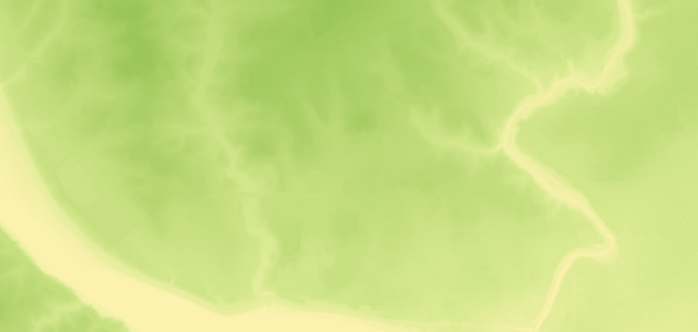
Color-relief (or hypsometric tint)

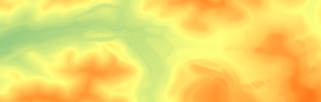
Color relief assigns a color to a pixel based on the elevation of that pixel. The result is not intended to be hysically accurate, and even if natural-looking colors are chosen the results should not be interpreted as representative of actual landcover. Low-lying areas are often given assigned green and yellow shades, with higher elevations blending to shades of grey, white, and/or red.

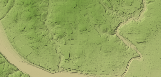
Hillshade (or shaded relief)

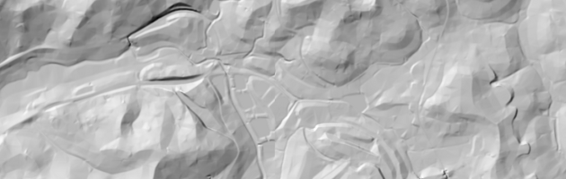
Hillshade visualization analyzes the digital elevation model to simulate a 3-dimensional terrain. The effect of sunlight on topography is not necessarily accurate but gives a good approximation of the terrain.

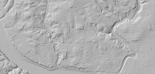
Slope

Slope visualization assigns a color to a pixel based on the difference in elevation between it and the pixels around it. We use it to make steep hills stand out and enhance the look of our terrain.

Visualizations with GDAL-DEM

Reprojecting the Data

Chances are your DEM datasource will not come in the Google Mercator projection we need - for example, SRTM comes as WGS84 (EPSG:4326) and USGS NED comes as NAD83 (EPSG:4269).

For our example we’ll be working with some NED data of the District of Columbia area. The following command will reproject the file to the proper projection - see Reprojecting a GeoTIFF for TileMill for more detailed information.

gdalwarp -s_srs EPSG:4269 -t_srs EPSG:3785 -r bilinear dc.tif dc-3785.tif

In the case of reprojecting elevation data, the -r bilinear option is important because other resampling methods tend to produce odd stripes or grids in the resulting image.

Creating hillshades

Run this command to generate the shaded relief image:

gdaldem hillshade -co compress=lzw dc-3785.tif dc-hillshade-3785.tif

The -co compress=lzw option will compress the TIFF. If you’re not concerned about disk space you can leave that part out. If you are using GDAL 1.8.0 or later you may also want to add the option -compute_edges in order to avoid a black pixel border around the edge of the image.

Our output looks like this:

Note: If there is not a 1:1 relation between your vertical and horizontal units, you will want to use the -s (scale) option to indicate the difference. Since Google Mercator X & Y units are meters, and NED elevation is also stored in meters this wasn’t necessary for our example. If your elevation data is stored in feet, you might do this instead (since there are approximately 3.28 feet in 1 meter):

gdaldem hillshade -s 3.28 -co compress=lzw dc-3785.tif dc-hillshade-3785.tif

Generating color-relief

Before you can create a color-relief image, you nee to decide what colors you want to assign to different elevations. This color configuration is created and stored in a specially formatted plain text file. Each line in the file should have four numbers - an elevation, and an RGB triplet of numbers from 0 to 255. To figure out the proper RGB values of a color, you can used the color selection tool of any image editor, or an online too such as ColorPicker.com.

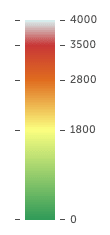
Here is our example, saved to a file called ramp.txt:

0 46 154 88
1800 251 255 128
2800 224 108 31
3500 200 55 55
4000 215 244 244

The above numbers define a gradient that will blend 5 colors over 4000 units of elevation. (Our units are meters, but we don’t need to specify that in the file.) They will translate to a color-to-elevation relationship that looks like this:

To apply this color ramp to the DEM, use the gdaldem color-relief command:

gdaldem color-relief input-dem.tif ramp.txt output-color-relief.tif

The area you are working with may not have such a wide range of elevations. You can check the minimum & maximum values of your DEM to adjust your ramp style accordingly. The gdalinfo command can tell us the range of values in the geotiff:

gdalinfo -stats your_file.tif

Among other things, this will tell you the minimum, maximum, and mean values of your elevation data to help you make decisions about how to choose your colors. With elevations tweaked for our area around DC, this is what we get:

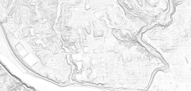
Generating slope shading

With the gdaldem tools, generating a slope visualization is a two step process.

First, we generate a slope tif where each pixel value is a degree, from 0 to 90, representing the slope of a given piece of land.

gdaldem slope dc-3785.tif dc-slope-3785.tif

The same note about horizontal and vertical scale as hillshades applies for slope.

The tif output by gdaldem slope has no color values assigned to pixels, but that can be achieved by feeding it through gdaldem color-relief with an appropriate ramp file.

Create a file called ‘slope-ramp.txt’ containing these two lines:

0 255 255 255
90 0 0 0

This file can then be referenced by by the color-relief command to display white where there is a slope of 0° (ie, flat) and display black where there is a 90° cliff (with angles in-between being various shades of grey). The command to do this is:

gdaldem color-relief -co compress=lzw dc-slope-3785.tif slope-ramp.txt dc-slopeshade-3785.tif

Which gives us:

Combining the final result in TileMill

To combine these geotiffs in TileMill, we’ll make use of the ‘multiply’ image blending mode using the raster-comp-op property, which stands for “compositing operation”. Assuming you have added your three geotiffs as layers with appropriate IDs, the following style will work. You can adjust the opacity of the hillshade and slope layers to tweak the style.

#color-relief,
#slope-shade,
#hill-shade {
    raster-scaling: bilinear;
    // note: in TileMill 0.9.x and earlier this is called raster-mode
    raster-comp-op: multiply;
}

#hill-shade { raster-opacity: 0.6; }

#slope-shade { raster-opacity: 0.4; }

The end result is something like this, ready to be combined with your vector data:

Raster performance

If your rasters are many MBs in size, then an important optimization is to build image pyramids, or overviews. This can be done with the gdaladdo tool or in QGIS. Building overviews does not impact the resolution of the original image, but it rather inserts new reduced resolution image references inside the original file that will be used in place of the full resolution data at low zoom levels. Any processing of the original image will likely drop any internal overviews previously built, so make sure to rebuild them if needed. You can use the gdalinfo tool to check if your tiff has overviews by ensuring the output has the ‘Overviews’ keyword reported for each band.