Optimizing shapefiles

If you've found yourself on this page, we're assuming you've

Set up GDAL

In this guide we will be downloading shapefiles from a single source, manipulating these to match a same map projection and optimizing these for performance in TileMill. To demonstrate how to alter a shapefile to use only what we need from it, I’ll cover how to create a custom layer from an existing source in step 3.

Downloading shapefiles across resources on the web will invariably be formatted differently. For consistency it’s a good idea to ensure they all conform to the single spatial reference system. For performance reasons, we’ll make sure this is the same as the final output SRS.

To get started, let’s download the ESRI shapefiles provide here: a collection of Shapefiles from Toronto http://toronto.ca/open.

Note for beginners: “ESRI shapefile” a popular format that is comprised of at least three separate files that must be kept together. Generally when using them with TileMill they are kept together in a zip archive. To manipulate them, we’re going to unzip them and once we have formatted the data for our purposes the files will be archived again and imported into TileMill. See the TileMill manual for more details.

##Tools

GDAL, an open source set of command line tools that let you quickly manipulate geospatial data. This will allow us to keep our shapefiles consistent by formatting them to the same spatial reference.
Quantum GIS, an open source Geographic Information System. For our purposes this will let us quickly load in shapefiles to preview the ones we want to use and create a custom one for our use in a map.

##Step 1. Map Projection

As a base layer, I’ll be using admin_0_countries.zip which is provided out of the box with TileMill. Its SRS is the same as TileMill’s output projection, Google Mercator (or ‘EPSG:900913’). By running a quick command we can see the SRS definitions of each shapefile we downloaded:

ogrinfo Neighbourhoods.shp -al -so The arguments -al and -so are flags to display this information as fields with sort order

The output of that command gives us this:

INFO: Open of `Neighbourhoods.shp'
      using driver `ESRI Shapefile' successful.

Layer name: Neighbourhoods
Geometry: Polygon
Feature Count: 140
Extent: (609544.138120, 4826145.039078) - (651617.899003, 4857223.341741)
Layer SRS WKT:
PROJCS["NAD_1927_UTM_Zone_17N",
    GEOGCS["GCS_North_American_1927",
        DATUM["North_American_Datum_1927",
            SPHEROID["Clarke_1866",6378206.4,294.9786982]],
        PRIMEM["Greenwich",0.0],
        UNIT["Degree",0.0174532925199433]],
    PROJECTION["Transverse_Mercator"],
    PARAMETER["False_Easting",500000.0],
    PARAMETER["False_Northing",0.0],
    PARAMETER["Central_Meridian",-81.0],
    PARAMETER["Scale_Factor",0.9996],
    PARAMETER["Latitude_Of_Origin",0.0],
    UNIT["Meter",1.0]]
DAUID: String (8.0)
PRUID: String (2.0)
CSDUID: String (7.0)
HOODNUM: Integer (4.0)
HOOD: String (33.0)
FULLHOOD: String (250.0)

The important line here is the Layer SRS WKT value, which is a well-known text definition of the SRS. The first value is a description: NAD_1927_UTM_Zone_17N, which is different from our base layer that has a value of Google_Maps_Global_Mercator. GDAL provides an extremely helpful command that will quickly convert this shape file into a new, specified srs. Here’s that command:

ogr2ogr formatted_neighbourhoods.shp Neighbourhoods.shp -t_srs EPSG:900913
To expand on this command we first state our output filename followed by the input filename (the file we wish to manipulate). -t_srs is the reproject/transform on output and ESPG:900913 is the code for the SRS we wish to set.

Now if we run ogrinfo formatted_neighbourhoods.shp -al -so our new file looks like this:

INFO: Open of `toronto_googled_neighbourhoods.shp'
      using driver `ESRI Shapefile' successful.

Layer name: formatted_neighbourhoods
Geometry: Polygon
Feature Count: 140
Extent: (-8865397.465252, 5400826.436911) - (-8807067.344161, 5443099.589880)
Layer SRS WKT:
PROJCS["Google_Maps_Global_Mercator",
    GEOGCS["GCS_WGS_1984",
        DATUM["WGS_1984",
            SPHEROID["WGS_1984",6378137,298.257223563]],
        PRIMEM["Greenwich",0],
        UNIT["Degree",0.017453292519943295]],
    PROJECTION["Mercator_2SP"],
    PARAMETER["standard_parallel_1",0],
    PARAMETER["latitude_of_origin",0],
    PARAMETER["central_meridian",0],
    PARAMETER["false_easting",0],
    PARAMETER["false_northing",0],
    UNIT["Meter",1]]
DAUID: String (8.0)
PRUID: String (2.0)
CSDUID: String (7.0)
HOODNUM: Integer (4.0)
HOOD: String (33.0)
FULLHOOD: String (250.0)

Quick tip: For a listing of all ogr2ogr supported formats you can type ogr2ogr --formats

##Step 2. Optimize with a shapeindex

There’s one last step I want to perform before I archive each of my shapefiles and import into a TileMill project. I will create an index file for Mapnik to utilize. There’s more on its performance benefits here.

shapeindex your-shapefile.shp

##Step 3. Create a custom layer

To give a geographical context to Toronto and its surroundings I want to include the lake of Ontario. Tilemill provides us with a lakes of the world shapefile lakes.zip out of the box but its more than what we need. I’m going to load this file into Quantum GIS and extract just the polygon of ontario lake as a geojson file. The GeoJSON format is great for this purpose as the data file is small and creating a file like this is quick and easy. See also this detailed tutorial on GeoJSON.

Here’s a quick rundown of those steps on a Mac:

Unzip lakes.zip
Import Lakes.shp into QGIS by selecting command-shift V. This key command will import vector layers.
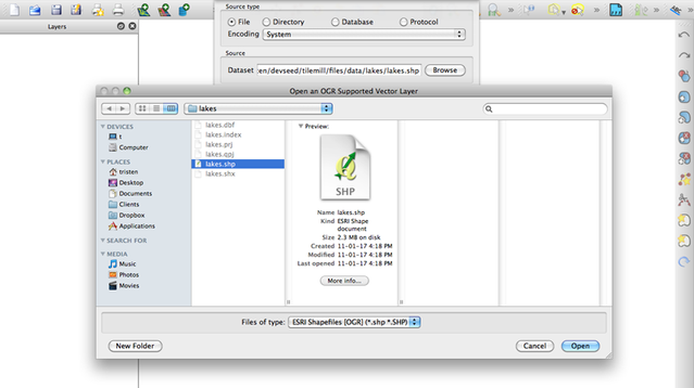
When the file has loaded into QGIS we should should see the polygons visually projected on the canvas. From the toolbar, press and hold the “Select Features” icon. Choose “Select Features by Polygon” to capture what I wish to use.
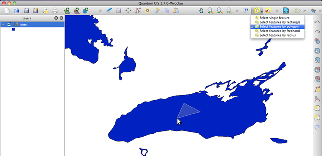
With the mouse over the selection, press ctrl and select to highlight a selection. I have now set a selection on Ontario to capture its polygon.
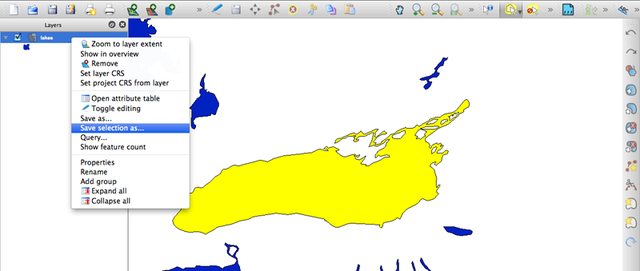
Finally, right select on lakes from the layers window and choose: “Save Section as”. Give this file a new name and save as .geojson.

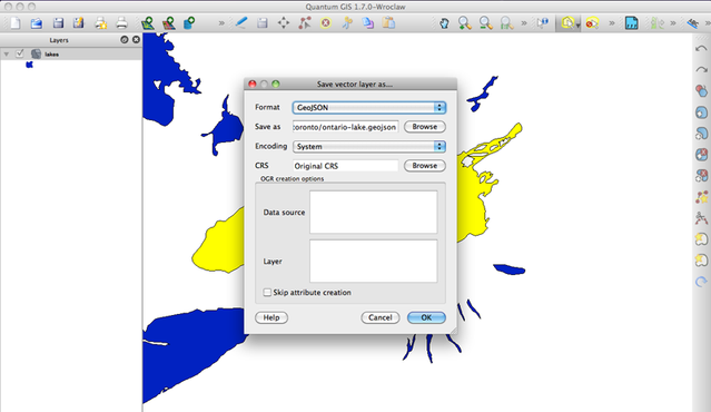
Alternatively, I could have saved this as an ESRI file, then ran ogrinfo and ogr2ogr. For simplicity sake let’s keep this as a .geojson file for now.

##Finished!

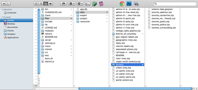
An optional step but with our new shapefiles I’ll package these neatly into a new directory called toronto.

At this point I am all set to begin designing in TileMill. Be sure to manually set the projection of your GeoJSON layer to 900913, as SRS autodetection is not yet functional for GeoJSON files. Happy Mapping!

Misson complete! Next up

Add a shapefile in TileMill.