Processing Landsat 8 Imagery

Note you will also need libgeotiff, to work with geotags (the tools used here are sometimes pagaged as ‘geotiff-bin’) and ImageMagick, an image processing package to complete the sections below.

Getting a scene

Download a scene from EarthExplorer, LandsatLook, or GLOVIS. You can use this helpful guide to EarthExplorer (credit: Robert Simmon), Note: If you find a lot of cloudy scenes for your area of interest, you can use a cloud coverage filter in the “Additional Criteria tab”.

In the bundle

The Level 1 Product comes as a .tar.gz file of about 700 megabytes to a gigabyte. Given the high demand for Landsat 8 imagery and the low funding for distribution infrastructure, you might want to get coffee while it downloads. (Note to Unix experts in a hurry: if you get the URL of the file, curl $URL | tar xfvz - will work.) The compressed file will unpack into a directory of 13 items, mostly TIFF images, each with an unwieldy-looking name starting with the 21-digit scene ID. This is the bundle. Here’s what you need to know about the bundle:

• The images with names ending in digits are the data for those bands. For example, LC80120542013154LGN00_B9.TIF is Band 9’s readout.

• The data is Level 1 terrain corrected, meaning that it’s been filtered to account for some sensor variations and for distortions caused by hills and valleys. The correction is not perfect, for example because the elevation dataset that it’s referenced against is a little coarse, but L1T is a good starting point for most uses.

• Each image is aligned with the others, so you know that a given pixel at x, y in one band’s data represents exactly the same point in space as the corresponding pixel in another image in the same bundle. The exception is Band 8, the pan band, which is at twice the linear resolution. (The alignment does not carry between different bundles that share path/row numbers. They can vary by 10 km or so.)

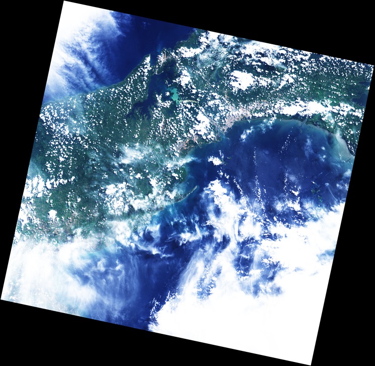
First draft true color

Landsat 8’s bands are explained in this blog post. The red, green, and blue bands are the ones numbered 4, 3, and 2. Re-project them to Google Web Mercator by:

for BAND in {4,3,2}; do gdalwarp -t_srs EPSG:3857 LC80120542013154LGN00_B$BAND.TIF $BAND-projected.tif; done

And merge them into an RGB image with convert:

convert -combine {4,3,2}-projected.tif RGB.tif

Incidentally, don’t worry when convert prints about a dozen warnings like this one:

convert: Unknown field with tag 33550 (0x830e) encountered. `TIFFReadDirectory' @ warning/tiff.c/TIFFWarnings/824.

ImageMagick is not geo-aware, and this is what it reports as it sees, and does not copy, geo fields. Steps to re-attach the geodata is mentioned below.

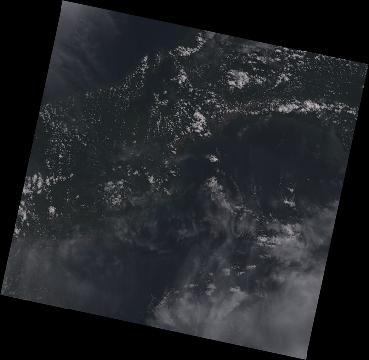
Truer color

By changing the brightness and contrast we can adjust the image to something that is closer to true color. One method is to use the -sigmoidal-contrast flag for convert, which takes a two-part argument: a scale factor for the contrast, plus the brightness value in the input image that should end up at 50% (midtone) in the output image. Run:

convert -sigmoidal-contrast 50x16% RGB.tif RGB-corrected.tif

Opening the output:

Using trial and error to find that the midtones in the input were at about 16% brightness in this image. If you want more consistent results, look in the file with the name ending MTL.txt, where you’ll find detailed records of optical attributes like sun angle, calibrated band radiances, and so on. If you’re doing further analysis, you’ll also get a lot of use out of the quality assurance pseudo-band, BQA.TIF, a bitfield in a format described here that helps find clouds, snow, missing data, etc.

There are textbooks on the topic of satellite image correction, but today we’ll keep it simple. We’ll account for haze by lowering the blue channel’s gamma (brightness) slightly, and raising the red channel’s even less, before increasing the contrast:

convert -channel B -gamma 0.925 -channel R -gamma 1.03 \ -channel RGB -sigmoidal-contrast 50x16% RGB.tif RGB-corrected.tif

This gives us something that’s green where it should be green:

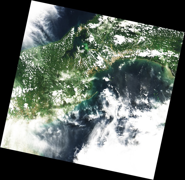
Like brightness and contrast, haze varies a lot between scenes, so take the numbers here as starting points for experimentation. If you want to turn the brightness way up to see lake surfaces better, or way down to see cloud structure, or run an edge detection filter to spot faint roadways, you can have at it. As long as you don’t change the dimensions of the image or introduce any spatial distortions, you can edit it from scratch however you please – with the full power of ImageMagick , with free or commerical graphical image editors, or with your own code – and you’ll still be able to re-attach the georeferences later.

False color (optional)

A true-color image is only one of the 165 distinct 3-band combinations that we can make from a single bundle, and not always the most informative one. If we’re interested in forest management and the water cycle, for example, we might want to look at the combination of NIR, SWIR, and visible red, using bands 5, 6, and 4 (similar to a 4-5-3 image from Landsat 5 or 7, for any old-timers in the audience). You can follow the same steps as you would for a 4-3-2 image, substituting the band numbers, then apply adjustments like these:

convert -channel B -gamma 1.25 -channel G -gamma 1.25 \ -channel RGB -sigmoidal-contrast 25x25% 564.tif 564-adj.tif

Those will bring out some contrast in the scene:

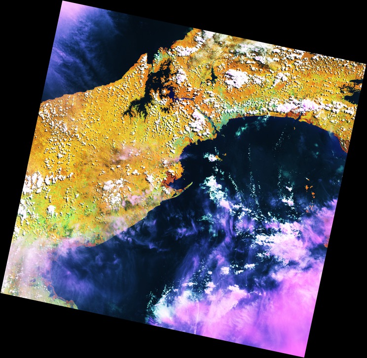
Now we can make general observations on topics like where there are mangrove swamps (brick-red areas), which we couldn’t see clearly in the true-color image.

A note of caution: all satellite images are somewhat processed by the time we see them. For false-color images in particular, there’s often a lot of adjustment to normalize the different bands. When doing anything important, it’s vital to understand exactly what you’re looking at, and only compare like with like. This image might give useful insights on certain topics, for example, but it would be a big mistake to compare it directly with an old Landsat 5 image using a similar band combination and assume that any apparent changes were real – unless you could be sure that they’d gone through exactly equivalent processing.

As well as direct combinations, at this stage you can apply cross-band transformations like NDVI, EVI, or tasseled cap. Anything that doesn’t change the spatial layout of the image will work.

Re-applying geodata

The processed image is a 16-bit TIFF without geodata, but we’d like an 8-bit TIFF with geodata. Changing the bit depth works like this:

convert -depth 8 RGB-corrected.tif RGB-corrected-8bit.tif

Since we were careful not to make any modifications that affected the spatial characteristics of the data (right?), we can copy the geographical information back from one of the projected but not manipulated bands. listgeo works well for this:

listgeo -tfw 4-projected.tif

It writes the geodata to a file with the same basename but the suffix .tfw (“TIFF worldfile”), which we’ll rename to match the file that we’re re-georeferencing:

mv 4-projected.tfw RGB-corrected-8bit.tfw

GDAL knows to look for a matching .tfw if it sees a TIFF that isn’t internally georeferenced, and while we’re at it will give the image a name that will be less confusing if it’s combined with other map elements:

gdal_edit.py -a_srs EPSG:3857 RGB-corrected-8bit.tif mv RGB-corrected-8bit.tif Panama-projected.tif

Importing to TileMill

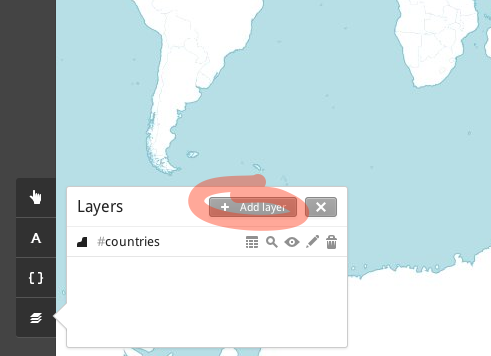
In a TileMill project, we add a layer via the menu at the bottom left:

And tell TileMill how to treat the image:

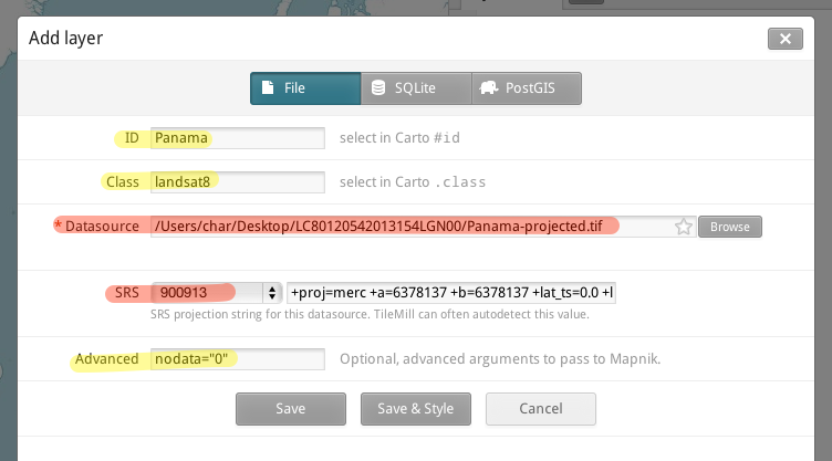
All TileMill really needs to know is where to find the image and what SRS to use. But giving it a useful ID and class makes it easier to work with as projects grow, and nodata="0" will make the black edges of the image transparent:

Now we have all the tools of TileMill at our disposal. You might be pulling in this image as one small part of a very complex project – but let’s keep this demo bare-bones and just set the raster-scaling method to lanczos, to help prevent jaggies.

Exporting from TileMill

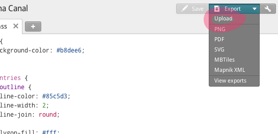
Once we’ve done everything we want in TileMill, we can use the Export menu in the upper right. We’ll upload to the MapBox account associated with TileMill (which can be changed in the Preferences screen):

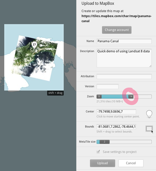
In the upload screen, we draw some reasonable boundaries and pick a center point. To save rendering time, let’s set the maximum resolution to zoom level 14, since that’s just beyond the maximum clarity that Landsat 8 could yield, even with pansharpening:

Once the tiles have rendered and uploaded, we have a browsable map hosted on MapBox:

Conclusions

We’ve downloaded Landsat 8 data, color-corrected it, pulled it into TileMill for use with other map resources, and uploaded it as a live map layer on MapBox. I hope this has encouraged you to make use of Landsat 8 data – and given you a head start on working with imagery from other sources.